


The mastery of sorting is an essential and critical skill for anyone seeking to excel in Data Structure and Algorithm, you cannot cheat the process! Let me tell you why.
I’m really glad to talk about this subject matter today because I’ve had quite a lot of awful experiences due to the lack of sorting algorithms during technical and live coding interviews and that’s why you should follow this series to the end in order to learn from my mistakes. Solving algorithmic questions can be quite challenging if you fail to understand the underlying principles and rudiments. It’s like studying music without a good knowledge of musical notes, which, in my opinion, would be one of the most expensive ways to learn music. In algorithms and coding in general, sorting is one of the essential instruments for writing them efficiently.
What’s Sorting, why does it matter?
Now that we are aware that sorting is one of the all-time foundational principles of data structures and algorithms, it is important not only to note that it involves arranging data items in a specific order but also different ways to implement it and putting consideration of efficiency and optimization. A deep understanding of sorting algorithms can help you as an engineer to optimize the performance of your code, improve search and retrieval times, and efficiently process large amounts of data when needed.
Throughout this post, we will be considering several sorting algorithms for arrays in ascending order.
Does Time & Space Complexity Matter?
Oh yes! Absolutely. Time and space complexity consideration in sorting algorithms matters as they both affect the outcome and performance of an operation. The time and space complexity is also dependent on various factors of the dataset, such as size, the distribution of data, available memory, and the computing power of the underlying operating system.
If you’re new to DSA and you’re wondering what time and space complexity is. They basically refer to the cumulative amount of time (iteration) and space (memory allocation) required to complete an algorithm. We will cover this topic in a future discussion
What are the types of Sorting?
There are many different types of sorting algorithms, each with its own strengths, weaknesses, and trade-off. Here is a list of some commonly used sorting algorithms:
- Bubble Sort:
It’s named after the way the largest element “bubbles” or “finds its way” to the top of the list with each pass of the algorithm. However, Bubble Sort is known for its inefficiency 😬, particularly for large data sets. Its time complexity is O(n²), which makes it impractical for sorting large data sets. Nevertheless, it is a simple algorithm to implement and can be useful for small data sets.
Here’s an example of how Bubble Sort works:
Consider an array = [5, 2, 4, 3, 1]. The first pass of Bubble Sort would compare the first two elements (5 and 2), swap them if they are in the wrong order, and then move to the next pair of adjacent elements. This process continues until the last two elements of the array have been compared, resulting in the largest element (5) being placed at the end of the array which is its final and correct position. The array is now [2, 4, 3, 1, 5] and that makes the end of the first pass. It starts the whole comparison over again for the second pass, from the first element (2), and starts searching the largest element through the remaining adjacent elements, this goes on and on until all the values in the array are properly placed in their correct position.
Two adjacent elements of an array are said to be in the wrong ascending order if the first element is greater than the second element
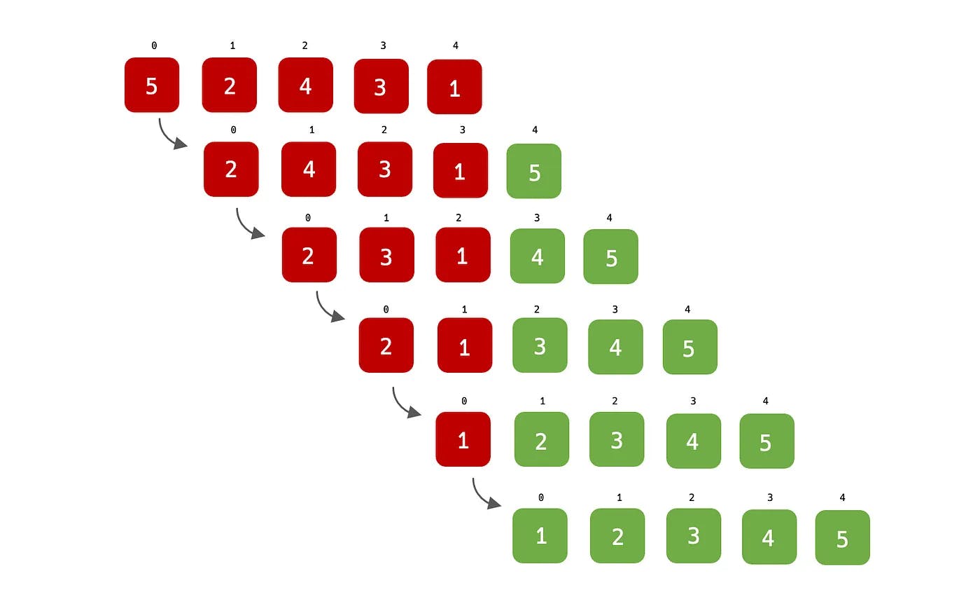
Please note that from the illustration above, each step represents an entire cycle of iteration or pass, and the sorting begins at the second step through the end, the red color signifies the item array that isn’t in its correct position, while the green shows the item that is correctly positioned. The time complexity for this algorithm is
O(n²)while the space complexity remains constant —O(1)
To remind us again, the logic behind this algorithm is to ensure that the largest value in array[i] at the nth iteration is placed to the left or right, depending on the sorting criteria i.e. ascending order, descending order and etc. Below is the sample code for Bubble Sort:
// Java
public static int[] bubbleSort(int[] array) {
    boolean isSorted = false;
    while(!isSorted) {
      isSorted = true;
      int index = 1;
      while(index < array.length) {
         if(array[index - 1] > array[index]) {
             isSorted = false;
             int temp = array[index - 1];
             array[index - 1] = array[index];
             array[index] = temp;
         }
         index++;
       }
    }
    return array;
 }

// Swift
 func static bubbleSort(_ array: inout [Int]) -> [Int] {
   var isSorted: Bool = false
   while(!isSorted) {
       isSorted = true
       var index = 1
       while(index < array.count) {
           if(array[index - 1] > array[index]) {
               isSorted = false
               (array[index - 1], array[index]) = (array[index], array[index - 1])
            }
            index += 1
        }
    }
    return array
 }

//Javascript
function bubbleSort(array) {
    let isSorted = false;
    while(!isSorted) {
        isSorted = true;
        let index = 1;
        while(index < array.length) {
            if(array[index - 1] > array[index]) {
                isSorted = false;
                [array[index - 1], array[index]] = [array[index], array[index - 1]];
            }
            index++;
        }
    }
    return array;
}

//C#
public static int[] BubbleSort(int[] array) {
    bool isSorted = false;
    while(!isSorted) {
        isSorted = true;
        int index = 1;
        while(index < array.Length) {
            if(array[index - 1] > array[index]) {
                isSorted = false;
                int temp = array[index - 1];
                array[index - 1] = array[index];
                array[index] = temp;
             }
             index++;
         }
     }
     return array;
}
2. Insertion Sort
It’s a simple sorting algorithm that builds the final sorted array one item at a time. It works by traversing an array of unsorted elements, removing one element at a time, and finding the correct position to insert it into the new sorted array.
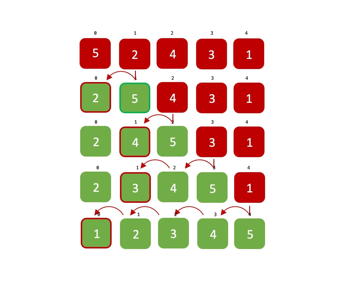
The arrow signifies the swapping of elements in the array that are not in order, and the example above demonstrates sorting in ascending order.
Let’s not make a fuss out of this algorithm. The simple explanation of this type of sorting algorithm is that we divide the array into two parts at every iteration. The first part is sorted, while the second part remains unsorted, then we pick the next item from the unsorted array and place it in the correct position of the sorted array. We repeat this operation until there is no unsorted part of the array left. Also, the time complexity of this algorithm is similar to that of Bubble sort O(n²) while its space complexity remains constant O(1).
A constant space complexity means that the size of the
arrayremains the same throughout the entire sorting operation.
With all of that being said, let’s now see how this is interpreted in code:
// Java
public static int[] insertionSort(int[] array) {
  for(int i = 1; i < array.length; i++) {
      int j = i;
      while(j > 0 && array[j] < array[j - 1]) {
        int temp = array[j];
        array[j] = array[j - 1];
        array[j - 1] = temp;
        j--;
      }
  }
  return array;
}

// Swift
func static insertionSort(_ array: inout [Int]) -> [Int] {
   for i in 1 ..< array.count {
     var j = i;
     while(j > 0 && array[j] < array[j - 1]) {
          array.swapAt(j, j - 1)
          j -= 1
      }
   }
   return array;
}

// Javascript
function insertionSort(array) {
    for(let i = 1; i < array.length; i++) {
        let j = i;
        while(j > 0 && array[j] < array[j - 1]) {
            [array[j], array[j - 1]] = [array[j - 1], array[j]];
            j--;
        }
    }
    return array;
}

// C#
public static int[] InsertionSort(int[] array) {
   for(int i = 1; i < array.Length; i++) {
       int j = i;
       while(j > 0 && array[j] < array[j - 1]) {
          int temp = array[j];
           array[j] = array[j - 1];
           array[j - 1] = temp;
           j--;
       }
    }
    return array;
}
If you look at the code carefully, you would notice that we started checking for comparison from array[1] towards the left-hand side, this is an important piece of insertion sort.
3. Quick Sort
Is a popular sorting algorithm that uses the divide-and-conquer strategy to sort an array. It works by selecting a “pivot” element from the array, and then partitioning the other elements into two sub-arrays, according to whether they are less than or greater than the pivot. The sub-arrays are then recursively sorted. What is interesting about quick sort is that the pivot element can be selected from any part of the array, the pivot element can be in the middle, outer-left and etc. In this example, we would be using theleft (LP) and right (RP) pointers, and we would be picking our pivot element from the middle. So imagine we have an array = [4, 3, 2, 5, 1], our pivot element is 2 and our LP and RP is 4 and 1 respectively. The main algorithm is to ensure that all the elements that are greater than the pivot value is moved to the right of the pivot, and elements that are lesser than the pivot value is moved to the left-hand side of the pivot value. We would ensure these rules are met until the LP index is greater than RP and then we exit the iteration. See the diagram below:
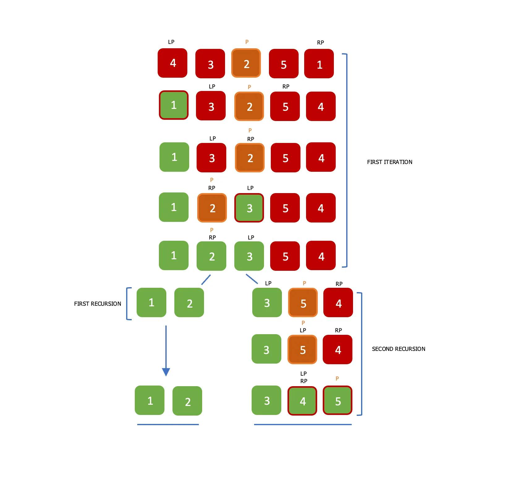
After the end of the first iteration, we would have to divide the array into two and perform the same quick sort operation recursively on each segment of the array, we will continue to do this until all the elements in the array are positioned in their final index. Let’s take a look at the code sample for a quick sort:
// -------------------- Java --------------------
class QuickSort {
    public static int[] quickSort(int[] array) {
          quickSort(array, 0, array.length - 1);
          return array;
    }

    public static void quickSort(int[] array, int start, int end) {
          if(start >= end) return ;
          int left = start, right = end;
          int pivot = array[(start + end) / 2];
          while(left <= right) {
              while(array[left] < pivot) {
                left++;
              }
              while(array[right] > pivot) {
                right--;
              }
              if(left <= right) {
                int temp = array[right];
                array[right] = array[left];
                array[left] = temp;
                left++; right--;
             }
          }
          quickSort(array, start, right);
          quickSort(array, left, end);
    }
}
// -------------------- Java ---------------------


// -------------------- Swift --------------------
class QuickSort {
    func quickSort(_ array: inout [Int]) -> [Int] {
        quickSort(&array, 0, array.count - 1)
        return array
    }

    func quickSort(_ array: inout[Int], _ start: Int, _ end: Int) {
        if(start >= end) { return }
        var left = start
        var right = end
        var pivot = array[(start + end) / 2]
        while (left <= right) {
          while(array[left] < pivot) { left += 1}
          while(array[right] > pivot) { right -= 1 }
          if(left <= right) {
            (array[left], array[right]) = (array[right], array[left])
            left += 1; right -= 1
          }
        }
        quickSort(&array, start, right)
        quickSort(&array, left, end)
    }
}
// -------------------- Swift --------------------


// ------------------ Javascript ------------------
var quickSort = (array) => {
      quickSortElement(array, 0, array.length - 1);
      return array;
}

var quickSortElement = (array, start, end) => {
      if(start >= end) { return ; }
      let left = start;
      let right = end;
      let pivot = array[Math.floor((start + end) / 2)];
      while (left <= right) {
          while(array[left] < pivot) { left++; }
          while(array[right] > pivot) { right--; }
          if(left <= right) {
              [array[left], array[right]] = [array[right], array[left]];
              left++; right--;
          }
      }
      quickSortElement(array, start, right);
      quickSortElement(array, left, end);
}
// ------------------ Javascript ------------------


// ---------------------- C# ----------------------
class QuickSort {
   public static int[] QuickSort(int[] array) {
        QuickSort(array, 0, array.Length - 1);
        return array;
    }

    public static void QuickSort(int[] array, int start, int end) {
        if(start >= end) { return; }
        int left = start;
        int right = end;
        int pivot = array[(start + end) / 2];
        while(left <= right) {
            while(array[left] < pivot) { left++; }
            while(array[right] > pivot) { right--; }
            if(left <= right) {
                int temp = array[left];
                array[left] = array[right];
                array[right] = temp;
                left++; right--;
            }
        }
        QuickSort(array, start, right);
        QuickSort(array, left, end);
    }
}
// ---------------------- C# ----------------------
In practice, quick-sort is often faster than both bubble sort and insertion sort, especially for large arrays. On average runtime, its time complexity is O(n log n) and a worst-case time complexity of O(n²), the standard space complexity for this sorting can be O(log n) while its worst-case would be O(n).
Conclusion
In conclusion, bubble sort, insertion sort, and quick sort are all sorting algorithms that can be used to sort elements in an array. Bubble sort is the simplest and easiest to implement, but it has a time complexity of O(n²) and is not efficient for large datasets. Insertion sort is also simple and efficient for small datasets, but it has a time complexity of O(n²) and is not well-suited for large datasets.
On the other hand, quick sort is generally the preferred choice for sorting large datasets, due to its average time complexity of O(n log n) and its ability to sort in place, requiring only a small amount of additional memory. However, quick sort can have a worst-case time complexity of O(n²) and can be unstable in some implementations.
Overall, the choice of sorting algorithm depends on the size and type of the dataset being sorted, as well as other factors such as the available memory and the specific requirements of the application. By understanding the strengths and weaknesses of each algorithm, developers can make informed decisions when it comes to choosing the right sorting algorithm for their use case.
Please stay tuned for the Part II 🙏